Explicit Euler Method
The explicit Euler method is by far the simplest numerical technique for solving ordinary differential equations. It has a clear geometric interpretation and is easy to apply. However, it is relatively rarely used because of its low accuracy.
It is called explicit because it does not require solving a nonlinear equation, unlike the implicit Euler method which will be introduced later.
Geometric Interpretation
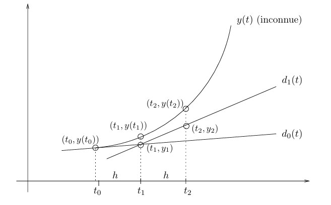
Consider the differential equation y′(t) = f(t, y(t)) with the initial condition y(t₀) = y₀. The goal is to obtain an approximation of the solution at t₁ = t₀ + h.
Before performing the first iteration, we need to determine the direction in which we must move from the point (t₀, y₀) to approximate the point (t₁, y(t₁)).
Although we do not know the exact curve y(t), we do know its slope at t = t₀, because:
y′(t₀) = f(t₀, y(t₀)) = f(t₀, y₀)
We follow the straight line passing through (t₀, y₀) with slope f(t₀, y₀). The equation of this line, denoted d₀(t), is:
d₀(t) = y₀ + f(t₀, y₀)(t − t₀)
Evaluating this at t₁ gives:
d₀(t₁) = y₀ + h f(t₀, y₀) = y₁
This value y₁ is an approximation of the exact value y(t₁):
y(t₁) ≈ y₁ = y₀ + h f(t₀, y₀)
In general, y₁ ≠ y(t₁), and this discrepancy affects all subsequent iterations.
Second Iteration and Error Propagation
To approximate y(t₂), we repeat the reasoning starting from the point (t₁, y₁).
The slope of the exact solution at t₁ is:
y′(t₁) = f(t₁, y(t₁))
Since y(t₁) is unknown, we use its approximation y₁:
f(t₁, y(t₁)) ≈ f(t₁, y₁)
We construct the line:
d₁(t) = y₁ + f(t₁, y₁)(t − t₁)
Then:
y(t₂) ≈ y₂ = y₁ + h f(t₁, y₁)
Remark
This development highlights an important property of numerical methods for solving differential equations: the error made in one iteration propagates into all subsequent iterations.
As a result, the quantity
| y(tₙ) − yₙ |
generally increases slightly as n grows.