Using the approach of the trapezoidal method but with a degree 2 polynomial passing through the points (x₀,f(x₀)), (x₁,f(x₁)), and (x₂,f(x₂)):
p₂(x) = f(x₀) + f[x₀,x₁](x−x₀) + f[x₀,x₁,x₂](x−x₀)(x−x₁)
The integral is approximated as:
∫x₀x₂ f(x) dx ≃ ∫x₀x₂ p₂(x) dx = ∫x₀x₂ { f(x₀) + f[x₀,x₁](x−x₀) + f[x₀,x₁,x₂](x−x₀)(x−x₁) } dx
For equally spaced points, using the change of variable (x−x₀)/h = s:
∫02 (f(x₀) + f[x₀,x₁] h s + f[x₀,x₁,x₂] h² s(s−1)) h ds = h/3 (f(x₀) + 4 f(x₁) + f(x₂))
Here, the divided differences are replaced by:
f[x₀,x₁] = (f(x₁)−f(x₀))/h , f[x₀,x₁,x₂] = (f(x₂)−2f(x₁)+f(x₀))/(2 h²)
Therefore, the simple Simpson 1/3 rule is:
∫x₀x₂ f(x) dx ≃ h/3 (f(x₀) + 4 f(x₁) + f(x₂))
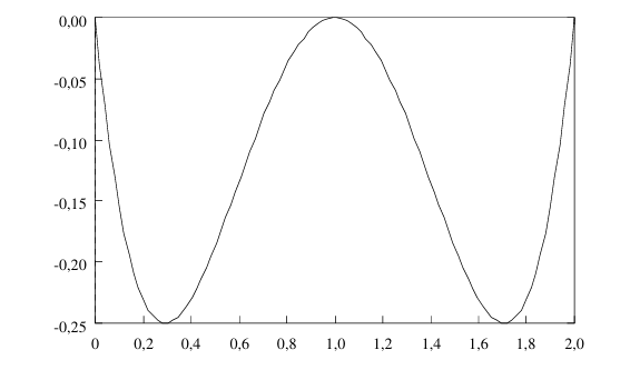
The error analysis shows that using a degree 2 polynomial actually provides the same precision as a degree 3 polynomial with a correction term through point x₃. By taking x₃ = x₁, the error term becomes:
∫x₀x₂ E₃(x) dx = f⁽⁴⁾(η)/4! ∫02 s(s−1)²(s−2) h⁵ ds = f⁽⁴⁾(η) h⁵ / 90 , η ∈ [x₀, x₂]
The simple Simpson 1/3 rule including the error is therefore:
∫x₀x₂ f(x) dx ≃ h/3 (f(x₀) + 4 f(x₁) + f(x₂)) − f⁽⁴⁾(η) h⁵ / 90
Remark: The value of h always represents the spacing between points xi, i.e., the interval length divided by 2. Choosing x₃ = x₁ ensures the polynomial remains well-defined.