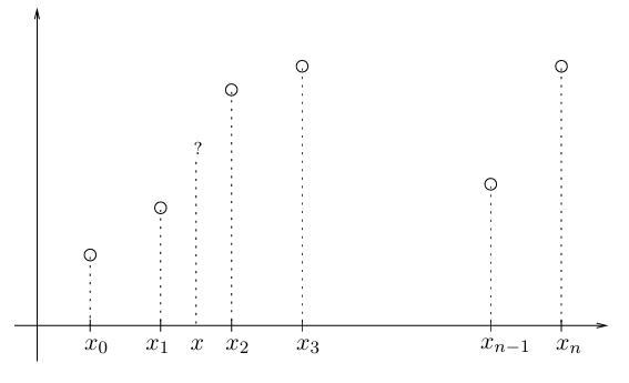
In many engineering and scientific problems, we often know the values of a function \( f(x) \) only at a limited number of discrete points \( (x_0, f(x_0)), (x_1, f(x_1)), \dots, (x_n, f(x_n)) \). The central question is: Can we construct an approximation of \( f(x) \) that is valid for any value of \( x \)?

The values \( x_i \) are called the interpolation nodes or sample points, while the pairs \( (x_i, f(x_i)) \) are known as collocation points. These points may come from experimental measurements, signal samples, or data tables.

In other words, when only a few discrete values of a function are available, we seek a mathematical procedure that allows us to estimate its value for any intermediate point not contained in the original dataset. This is the essence of interpolation.

The goal of polynomial interpolation is to find a polynomial of sufficiently high degree whose curve passes through all the known data points. Such a polynomial is called the interpolating polynomial or collocation polynomial.

Once the interpolating polynomial is constructed, it becomes a powerful tool: we can easily compute approximate values of the function at unsampled points, visualize its general behavior, and perform further analysis such as differentiation or integration if needed.

Polynomial interpolation plays a fundamental role in many applied fields, such as:

• Signal processing — reconstructing missing or noisy samples from discrete signals.
• Data compression — representing continuous signals by a limited set of interpolation coefficients.
• Numerical modeling — estimating unknown functional values in simulations or experiments.
• Control and communication systems — approximating transfer functions or responses based on sample data.