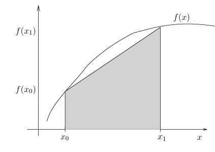
Let us begin with the simplest method. We want to evaluate:

∫_x₀^x₁ f(x) dx

where f(x) is known only at two points, or is a function without a primitive. The immediate solution is to replace f(x) by the degree 1 polynomial passing through the points (x₀,f(x₀)) and (x₁,f(x₁)), as illustrated in the figure.

The approximate value of the integral corresponds to the area under the polynomial curve. This area forms a trapezoid, giving its name to the trapezoidal method. Obviously, this approximation is coarse and is likely to be of limited precision. Using Newton's polynomial and the error relation, we have:

∫_x₀^x₁ f(x) dx = ∫_x₀^x₁ p₁(x) dx + ∫_x₀^x₁ E₁(x) dx = ∫_x₀^x₁ { f(x₀) + f[x₀,x₁](x − x₀) } dx + ∫_x₀^x₁ f″(ξ(x)) / 2! (x − x₀)(x − x₁) dx

Integrating the polynomial, we get:

∫_x₀^x₁ f(x) dx = (x₁−x₀)/2 (f(x₀) + f(x₁)) + ∫_x₀^x₁ f″(ξ(x)) / 2! (x − x₀)(x − x₁) dx

The first term on the right-hand side represents the trapezoid area, while the second term is the error. Using the change of variable s = (x−x₀)/h, we have dx = h ds and (x−xᵢ) = (s−i)h, leading to:

∫_x₀^x₁ f″(ξ(x)) / 2! (x − x₀)(x − x₁) dx = ∫₀¹ f″(ξ(s)) / 2! s(s − 1) h³ ds

Applying the second mean value theorem for integrals:

∫_a^b f₁(x) f₂(x) dx = f₁(η) ∫_a^b f₂(x) dx, η ∈ [a,b]

Since s(s−1) does not change sign in [0,1], there exists η ∈ [0,1] such that:

∫₀¹ f″(ξ(s)) / 2! s(s−1) h³ ds = f″(η) / 2! h³

Therefore, the trapezoidal method can be summarized as:

∫_x₀^x₁ f(x) dx = h / 2 (f(x₀) + f(x₁)) − f″(η) / 12 h³, η ∈ [x₀, x₁]