UF-70569-M1-S1-FINBAN: Lecture 5: Calculating Return and Risk for a Portfolio Composed of N Financial Assets:

Lecture 5: Calculating Return and Risk for a Portfolio of N Financial Assets

1. Expanding the Concept of Return and Risk to Include Portfolios with More Than Two Assets

When dealing with portfolios composed of $N$ financial assets, the same principles of expected return and risk apply but are generalized to account for multiple assets. The calculations become more complex due to the interactions (covariances) between all pairs of assets.

Expected Return of the Portfolio :
The expected return of a portfolio is still the weighted average of the expected returns of the individual assets.

$E (R_{p}) = i = 1 \sum N w_{i} \cdot E (R_{i})$
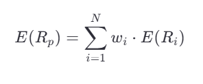
Where:
$E (R_{p})$ : Expected return of the portfolio
$w_{i}$ : Weight of asset $i$ in the portfolio
$E (R_{i})$ : Expected return of asset $i$
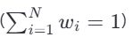
Portfolio Variance :
The variance of the portfolio depends on the variances of the individual assets, their covariances, and the weights assigned to them. For $N$ assets, the formula expands as follows:

2. Using Matrices to Calculate Portfolio Variance and Standard Deviation

For large portfolios ( $N > 2$ ), matrix algebra simplifies the computation of portfolio variance.

Matrix Representation :
Let:
$W = [w_{1}, w_{2}, ..., w_{N}]^{T}$ : A column vector of asset weights
$Σ$ : The covariance matrix of size $N \times N$ , where each element represents $Cov (R_{i}, R_{j})$ .

The portfolio variance can be written as:

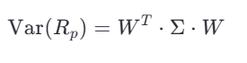
Where:

$W^{T}$ : Transpose of the weight vector
$Σ$ : Covariance matrix

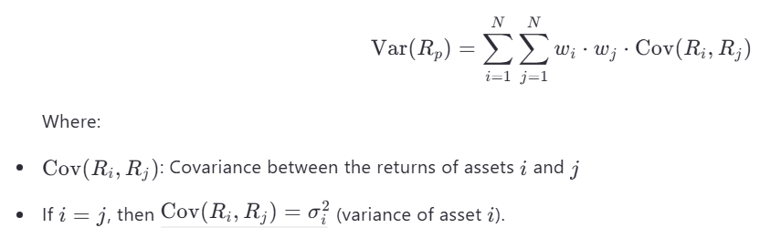
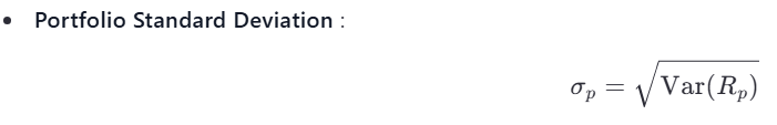
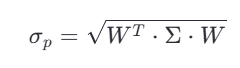
The portfolio standard deviation is then:

3. Including the Risk-Free Asset and Its Impact on the Portfolio

A risk-free asset (e.g., government bonds or treasury bills) has zero risk ( $σ_{f} = 0$ ) and is uncorrelated with risky assets. Including a risk-free asset in the portfolio changes the calculation of return and risk:

Expected Return of the Portfolio with a Risk-Free Asset :
If a portion of the portfolio is invested in a risk-free asset with return $R_{f}$ , the expected return of the portfolio becomes: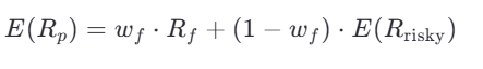

Where:
$w_{f}$ : Weight of the risk-free asset
$E (R_{risky})$ : Expected return of the risky portfolio
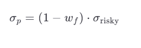
Portfolio Risk with a Risk-Free Asset :
Since the risk-free asset has no variance or covariance with risky assets, the portfolio's total risk depends only on the risky portion:
Capital Allocation Line (CAL) :
The inclusion of a risk-free asset allows investors to create portfolios along the Capital Allocation Line, which represents combinations of the risk-free asset and the optimal risky portfolio.

4. Practical Examples and Calculations

Example 1: Expected Return and Variance of a Portfolio with 3 Assets

Suppose you have a portfolio with three assets:

Asset 1: $E (R_{1}) = 8%$ , $σ_{1} = 10%$
Asset 2: $E (R_{2}) = 12%$ , $σ_{2} = 15%$
Asset 3: $E (R_{3}) = 10%$ , $σ_{3} = 12%$
Weights: $w_{1} = 40%$ , $w_{2} = 30%$ , $w_{3} = 30%$
Covariances:
- $Cov (R_{1}, R_{2}) = 0.006$
- $Cov (R_{1}, R_{3}) = 0.004$
- $Cov (R_{2}, R_{3}) = 0.009$

Step 1: Calculate Expected Return

$E (R_{p}) = (0.4 \cdot 8%) + (0.3 \cdot 12%) + (0.3 \cdot 10%) = 3.2% + 3.6% + 3.0% = 9.8%$

Step 2: Calculate Portfolio Variance

$Var (R_{p}) = (0. 4^{2} \cdot 0. 1^{2}) + (0. 3^{2} \cdot 0.1 5^{2}) + (0. 3^{2} \cdot 0.1 2^{2}) + (2 \cdot 0.4 \cdot 0.3 \cdot 0.006) + (2 \cdot 0.4 \cdot 0.3 \cdot 0.004) + (2 \cdot 0.3 \cdot 0.3 \cdot 0.009)$

$Var (R_{p}) = 0.0016 + 0.002025 + 0.001296 + 0.00144 + 0.00096 + 0.00162$

$= 0.008941$

Step 3: Calculate Portfolio Standard Deviation

Example 2: Including a Risk-Free Asset

Suppose the portfolio from Example 1 is combined with a risk-free asset with $R_{f} = 4%$ and $w_{f} = 30%$ .

Step 1: Calculate Expected Return

$E (R_{p}) = (0.3 \cdot 4%) + (0.7 \cdot 9.8%) = 1.2% + 6.86% = 8.06%$

Step 2: Calculate Portfolio Risk

$σ_{p} = (1 - 0.3) \cdot 9.46% = 0.7 \cdot 9.46% \approx 6.62%$

Key Takeaways

Generalization : The concepts of expected return and risk extend to portfolios with $N$ assets using weighted averages and covariance matrices.
Matrix Algebra : Matrix representation simplifies variance calculations for large portfolios.
Risk-Free Asset: Including a risk-free asset reduces portfolio risk while allowing for strategic allocation along the Capital Allocation Line.
Practical Application: These tools enable investors to optimize portfolios with multiple assets and achieve better risk-return trade-offs.

Modifié le: vendredi 11 juillet 2025, 00:32

إدارة المحافظ المالية/ Portfolio ManagementLecture 5: Calculating Return and Risk for a Portfolio Composed of N Financial Assets:

Lecture 5: Calculating Return and Risk for a Portfolio of N Financial Assets

1. Expanding the Concept of Return and Risk to Include Portfolios with More Than Two Assets

E(Rp​)=i=1∑N​wi​⋅E(Ri​)

2. Using Matrices to Calculate Portfolio Variance and Standard Deviation

3. Including the Risk-Free Asset and Its Impact on the Portfolio

4. Practical Examples and Calculations

Example 1: Expected Return and Variance of a Portfolio with 3 Assets

E(Rp​)=(0.4⋅8%)+(0.3⋅12%)+(0.3⋅10%)=3.2%+3.6%+3.0%=9.8%

Var(Rp​)=(0.42⋅0.12)+(0.32⋅0.152)+(0.32⋅0.122)+(2⋅0.4⋅0.3⋅0.006)+(2⋅0.4⋅0.3⋅0.004)+(2⋅0.3⋅0.3⋅0.009)

Var(Rp​)=0.0016+0.002025+0.001296+0.00144+0.00096+0.00162

=0.008941